Improving A Multiple Linear Regression Model For Predicting Route Quality

Introduction

In my previous post we constructed a simple multiple linear regression model for predicting climbing route quality. It wasn’t an awful effort, but there are many avenues for improvement. In particular:

1. Cross-Validation. Previously, we gauged our model effectiveness by simply considering our training R-Squared, which is an easy way to end up with an overfit model and subsequently get clobbered when trying to apply the model to new test data. We will use cross validation with a hold-out test set to yield a model that performs well when exposed to new data.
2. Improved Data Cleaning. We learned a lot about how to clean our features last time, but we can do even better using better informed imputation, category encoding, and scaling methods.
3. Interaction and Higher Order Features. Introduce 2nd order and interaction terms for our features. Control over-fitting here with subsequent feature selection.
4. Feature Selection. We can attempt stepwise, L2 regularization, mutual information, and partial least squares to improve our feature selection.
5. Regularization. We can use ridge, lasso, and elastic net regression to regularize our model to prevent over-fitting.
6. Outlier Resistant Loss Functions We can use methods such as Huber Regression to reduce the impact of outliers.

Throughout this project, we learn the following things:

• How to decide on imputation, categorical encoding and scaling methods.
• How to implement pipelines to minimize data leakage.
• How to perform cross-validated grid searches to optimize parameters.
• How to integrate preprocessing parameters into our pipeline.
• How to use a variety of techniques to best select features.
• What techniques to avoid on the basis of excessive computational overhead.

Data Introduction

This section is mostly taken from my previous post and is intended to give context to those reading just this post.

I’ve scraped all non-boulder routes from Mountain Project, amounting to n=30,738 routes, for the following locations:

Bishop Area, Black Canyon of the Gunnison, Eldorado Canyon, High Sierra, Index, Indian Creek, Joshua Tree, Lake Tahoe, Leavenworth, Mammoth Lakes, Moab Area, New River Gorge, Red River Gorge, Red Rock, Rifle, Rumney, Smith Rock, Squamish, Ten Sleep, The Needles (CA), Tuolomne, Vedauwoo, Yosemite, Zion.

We begin with p=16 features, though it is likely we will drop some. Since p«n, we are lucky enough to be far and away from a p»n or even p~n case which requires special care when constructing a model.

Selecting a Response Variable

Creating a meaningful summary metric for quality given a series of votes is not an uncommon problem to have. The first thing that typically comes to mind is to use a simple arithmetic mean, which isn’t a bad idea, but it does not do a very good job of accounting for a difference in number of votes. An item with 1x5star review will be ranked higher than an item with 999x5star reviews and 1x1star review. A statisticians perspective says to consider your pool of votes to be a sampled subset of your true population, which can be used to estimate the true population value. It depends, like most things in statistics, on the number of samples. It is important to note that we are not saying items with low vote counts are inherently worse, but we are less certain of their true state. By using this concept we build a list that is our proposed “best guess” estimate of the ranking.

Before we select a model, we should be aware of what information is available to us. I have access only to the average rating and number of ratings. I do not have access to the individual ratings.

The Wilson Score Interval is a favorite among binomial ranking systems such as Reddit’s upvote/downvote system. It can be modified to work with more than two options. Unfortunately because my data set does not have the individual rankings, I cannot make use of this method. Besides, there has to be a more relevant method for a star ranking system like we have here.

Companies like Amazon and IMBD surely care about ranking items with a star system. It is possible they are using a more complicated method overall, but the typical basis seems to be the Bayesian Average Ref Ref. In short, it assumes the default rating for an item is the mean of the entire set, this is ‘m’. Then as votes are added that value is adjusted accordingly. How many votes are required to be confident of the true value is ‘C’, which is based on the number of votes. This is more nuanced to select. Some people use the mean, some use the 25th percentile. We have the required components to construct this new metric.

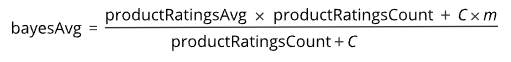Bayes Average Equation [Source]

We just need to select ‘C’. A percentile plot shows our rather skewed distribution nicely.

This is where we make a rather large decision. A common standard is 25th percentile, which here is 2. However, I simply do not believe that a route rating with less than 5 votes is anywhere near accurate. Additionally, we will be using metrics calculated from additional user submitted data for each route, and routes with low rating votes are likely to have minimal or even missing data for these metrics. If we remove all entries with <5 votes, we will be removing *44%! of the data. This is a huge hit. It will also make our model worse at predicting these lesser known routes. We will however, be minimizing the amount of unconfident noisy data in our model. To keep our model simple, it is a good idea to limit our scope and focus on items we have meaningful data for. Further attunements to that end can come later.

Removing these values and taking C to be the 25th percentile yields a value of 9. This is reasonable.

Calculating the Bayesian Stars is very simple.

m = df['Avg Stars'].mean()
c = df['Num Star Ratings'].quantile(0.25)
df['Bayesian Stars'] = ((df['Avg Stars'] * df['Num Star Ratings']) + (c*m)) / (df['Num Star Ratings'] + c)

Let’s check out what this transformation has done to our rating distribution.

So we removed all routes with missing “Avg Stars” and “Num Star Ratings”. We also removed all routes with <5 “Num Star Ratings”. This reduced our data set from 30,738 to 14,964, a reduction of 51%.

A typical shorthand explanation of the star system for climbs is as follows:

• 0-1 : likely junk, not worth your time.
• 1-2 : A fine climb, worth your time but likely not remarkable.
• 2-3 : An area classic, likely very good.
• 3-4 : An all time classic, likely excellent.

Feature Descriptions

Start by checking the head and seeing what we are working with.

	Route ID	Route	Location	Area Latitude	Area Longitude	Route Type	Rating	Risk	Length	Pitches	SP/MP	Num Ticks	Num Tickers	Lead Ratio	OS Ratio	Repeat Sender Ratio	Mean Attempts To RP	Bayesian Rating
14067	105717901	Astro Lad	Wall Street > Potash Road > Southeast Utah > Utah	38.54668	-109.59959	Trad	5.11a	NaN	60.0	1	SP	254.0	209.0	0.692771	0.454545	1.045455	1.400000	3.543581
28317	107290449	Blind Faith	Ba. The Rostrum > Lower Merced River Canyon > ...	37.71848	-119.70799	Trad	5.11+	NaN	400.0	5	MP	37.0	32.0	0.714286	0.928571	1.000000	1.000000	3.615288
16044	106580254	Ledgends of Limonite	The Great Wall > Muir Valley > Red River Gorge...	37.73288	-83.63751	Sport	5.8	NaN	55.0	1	SP	716.0	639.0	0.773960	0.834286	1.037855	1.259259	2.128985
2117	105749890	Werk Supp	The Bastille - N Face > The Bastille > Eldorad...	39.93070	-105.28300	Trad	5.9	NaN	200.0	2	MP	2423.0	1454.0	0.679305	0.654577	1.230958	2.050847	3.391432
4278	107619457	Fairy Dust	Cliffs of Insanity > Indian Creek > Southeast ...	38.15145	-109.59834	Trad	5.11-	NaN	70.0	1	SP	6.0	6.0	0.666667	1.000000	1.000000	NaN	2.619470

Route ID - Int. Primary key. Unique. Extracted from URL.

Route - String. Name of route. high cardinality but not necessarily unique. Likely not a particularly useful predictor, but an important human-interpretable reference for talking about any specific entry.

Location - String. Series of sub-locations listed from “leaf” to “root”. Useful to create categorical groupings of entries in close proximity.

Area Latitude - Float. Latitude of terminal sub-location. Useful for plotting geo-spatial data. Likely high correlation with leaf of location string.

Area Longitude - Float. Longitude of terminal sub-location. Same comment as for latitude.

Route Type - Binary Categorical String. Style of climbing protection offered on route. Either “Trad” or “Sport”.

Rating - Categorical String. Designates consensus difficulty of climb. Uses Yosemite Decimal System. Designates consensus difficulty of climb.

Risk - Categorical String. Designates lack of protection on route, and consequence for a fall. Uses movie theater style ratings. If a fall occurs, “PG13” suggests injury, “R” suggests serious injury or maiming, “X” suggests death.

Length - Float. Length of route measured in feet.

Pitches - Int. Number of pitches the route is typically segmented into. Likely high correlation with “Length”.

SP/MP - Binary Categorical String. Designates whether the climb is a single pitch (“SP”), or multiple pitches (“MP”). Likely high correlation with “Length” and “Pitches”. An additional useful predictor as the difference in style and surrounding predictor data quality vary drastically between the two groups.

Num Ticks - Int. Number of user submitted ticks. A tick is a record of a climbers attempt on a route, including the date, style, success outcome, and comment. A measure of popularity and data integrity of metrics derived from tick data.

Num Tickers - Int. Number of users who submitted ticks. Since a user can submit multiple ticks for the same route, this provides an indirect measure of how many people return to a route. Likely high correlation with “Num Ticks”

Lead Ratio - Float. Ratio of ticks that claim to have led the route as opposed to top-rope or follow. A measure of many potential things: “Scary-ness” of route, difficulty to set up top-rope, inconvenience of following etc.

OS Ratio - Float. Ratio of ticks that claim to onsighted the route as opposed to a fell/hung or redpoint. A secondary measure of difficulty, or “tricky-ness”.

Repeat Sender Ratio - Float. Average number of times a climber who has redpointed or onsighted the route has returned for another clean send. this includes the first redpoint so there is a minimum value of 1. A measure of popularity.

Mean Attempt To RP - Float. Average number of attempts to achieve a redpoint. This includes the redpoint attempt itself so there is a minimum value of 1. A measure of difficulty to “work” a route clean.

Cross Validation

We are going to employ “Hold-Out” cross validation, wherein we perform a standard training/test split of 90-10. The 90% training split goes to cross-validation which is utilized to find optimal parameters for the model. The model is then applied to the 10% hold-out test split to yield error metric by which we can assess model performance.

The cross-validation set is itself split into multiple test and training split. There exists Leave One Out Cross-Validation (LOOCV) which is typically not preferred as it requires fitting and predicting the model n times. We will be using k-fold CV with k=5 for computational efficiency.

It is important that we utilize a proper pipeline, so to avoid data leakage that can occur if we utilize test data to train our model. This means employing a proper test-train split pipeline within our cross-validation, then performing a second summary test-train split pipeline between our entire cross-validation set and our hold-out test set.

This idea is well represented in the following graphic:

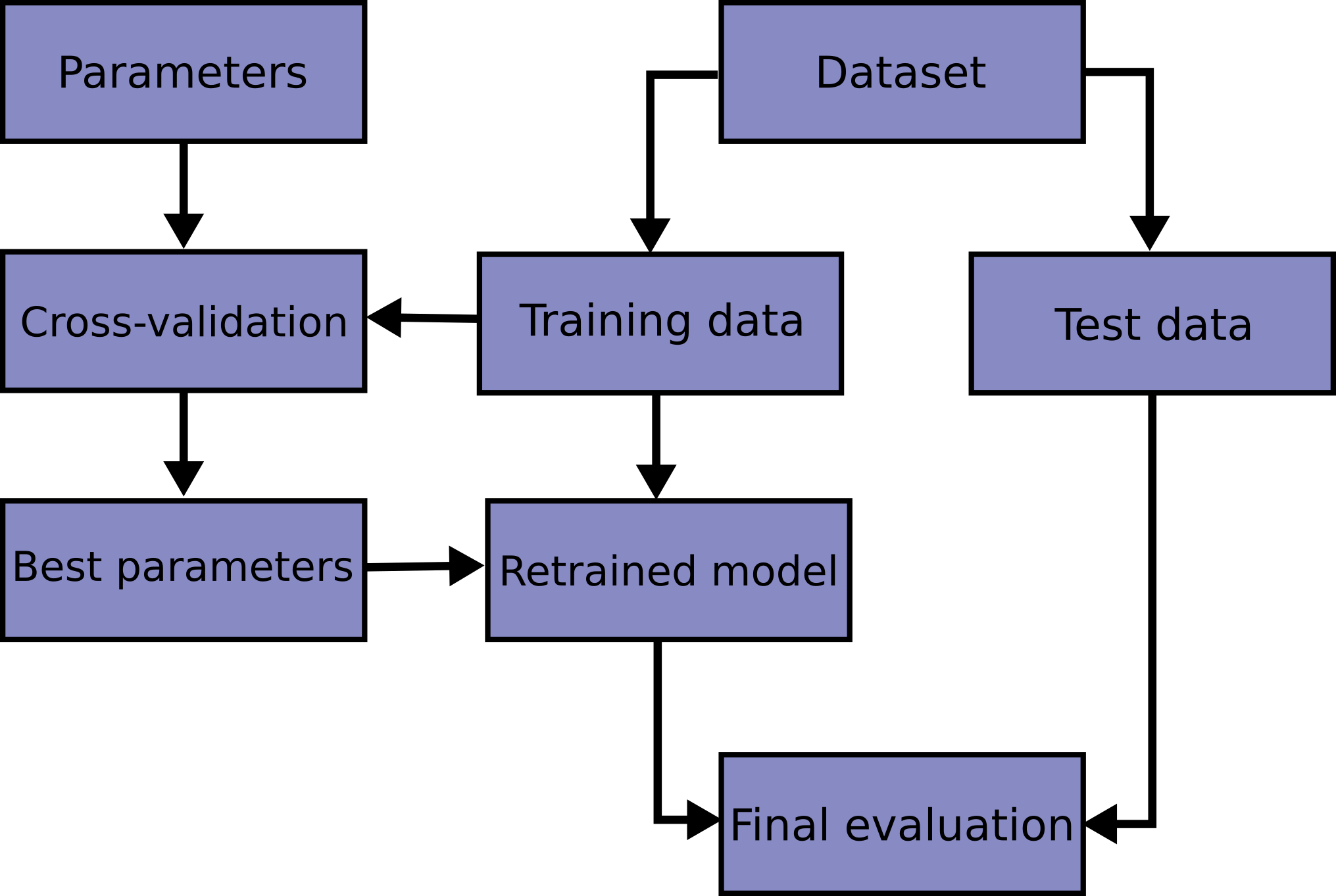Typical Cross Validation Pipeline [source]

Data Cleaning

We are going to reduce our dataset such that it only contains single pitch climbs by removing all multi-pitch entries. This is because many of the features have unclear or highly variable interpretations for multi-pitch climbs. This is inherent to the source of our data. I believe we can construct a more limited, but more effective model this way. As a result we will be dropping the “SP/MP” and “Pitches” features as they are now the same value across all entries. This reduces our sample size from 14,964 to 12,990. A Reduction of 13%.

We will also drop the “Num Tickers” feature as it has high collinearity with “Num Ticks” as ascertained previously through pearson’s correlation and variance inflation factor (VIF).

We will also be dropping the “Location” feature to avoid a headache inducing categorical encoding. Instead we can potentially leverage the “latitude” and “longitude” features to yield similar, but more easily handled, information value. This particularly benefits us as we can avoid more complex categorical encoding schemes. We need to remain wary that none of these linear regression models will be able to account for an XOR relationship. It is likely that the best information may be yielded from these features by a model that can handle such a relationship, such as a tree based model. I am wary of including these features from the get-go for that reason.

Imputation

We can explore the severity of null-values within our dataset using missingno plots.

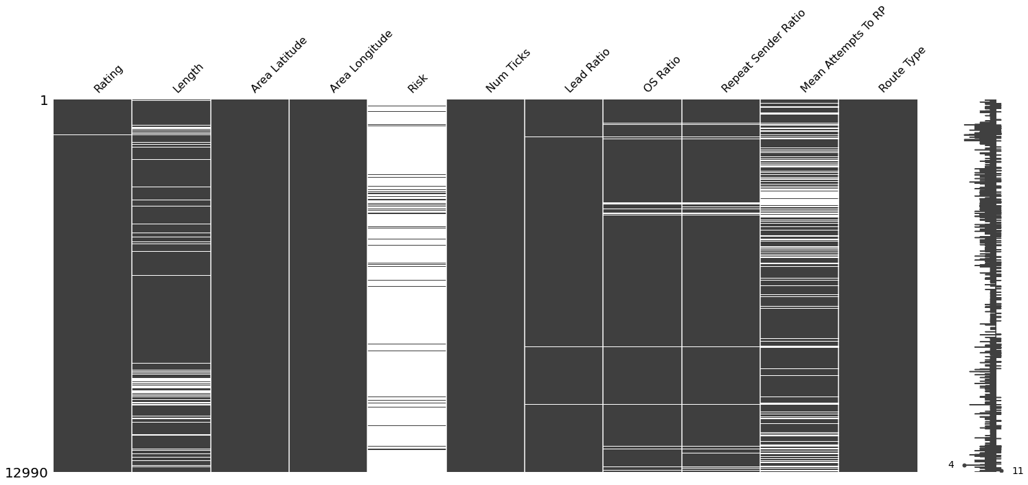Null Matrix Plot

Null Correlation Plot

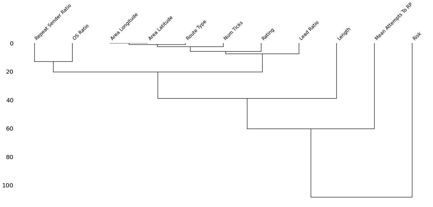Null Dendrogram

Feature	Percent Null
Rating	0.25
Length	11.04
Area Latitude	0.00
Area Longitude	0.00
Risk	93.94
Num Ticks	0.05
Lead Ratio	0.40
OS Ratio	2.61
Repeat Sender Ratio	3.90
Mean Attempts To RP	28.22
Route Type	0.01

We can see that Rating, Num Ticks, and Route Type all have only a small handful of null values. From the correlation and dendrogram plots we can see that there is a nominal amount of nullity correlation. Upon inspection we see that these entries are typically ridge traverses which are not particularly relevant to our analysis. These entries can be soundly dropped. This reduces our sample size from 12,990 to 12,946. A reduction of 0.3%.

Risk has many null values. In this case, the null value actually has a consistent and clear meaning. It designates the lack of a risk factor, in effect a “G” rating. These can be constant simple imputed.

I am confident that the remaining null containing features are “Missing at Random” (MAR) as opposed to Missing Completely at Random (MCAR) or Missing Not at Random (MNAR). If I thought they were MCAR, we would have much more flexibility as to which imputation method we could use and still obtain a sound model. I believe these missing values are somewhat dependent on other features that I have data for. For length this would be length itself of nearby routes as measured in latitude and longitude. The rest of the features are dependent in large part by number of ticks and likely in some part by all other features. If we were MNAR, then our null values likely depend on another feature for which we do not have data for. In this case even more complex imputation would yield an under-performant model. Though it is unlikely we have all relevant features to make a fully optimal regression, I do believe we have a good foundation.

Length imputation I handled in depth in my previous post. In short we are using a modified regression imputation that depends specifically on locally grouped length data and pitch number only. This is in contrast to a less directed regression imputation which likely contains many more variables. This decision was based on certain domain knowledge that these are far and away the most important factors. We may want to implement a form of stochastic regression by including some random variance based on the local group data. This would help to reduce the bias and under-estimatation of RMSE in our model that arises due to these more basic imputation methods.

This leaves four features of particular concern: Lead Ratio, OS Ratio, Repeat Sender Ratio, and Mean Attempts To RP. All of these metrics depend on submitted tick data for the individual route. This tick data is a better estimation of the true parameters of the climb when more ticks or present, which is typically more true if a climb is popular. Of the features, OS Ratio and Repeat Sender Ratio have very heavy null correlation, which is sensible given that Repeat Sender Ratio essentially counts repeated onsights (or redpoints which accounts for the imperfect correlation). Additionally, Mean Attempts To RP has particularly high nullity. Enough so, that I would consider dropping the Mean Attempts To RP feature entirely. For now we will keep it, but I’d like to keep an eye on it.

For these features it may be best to use “Multiple Imputation” AKA “Multivariate Imputation by Chained Equations” AKA MICE. This imputation method is heavily preferred by those concerned with measuring uncertainty in the model as it minimizes bias and error under-estimation in our model. Where stochastic regression is a band-aid, this is a proper solution. This along with “Maximum Likelihood Imputation” (of either an “Expected Maximization” or “Full Information Maximum Likelihood” type) are options. The details of which can be found in Ch.1 of Applied Missing Data Analysis by Craig Enders. Multiple imputation has an implementation in Scikit-Learn using “IterativeImputer”.

Another important option to make here is whether or not to include a “Missing Value” feature that designates which entries were imputed. It is possible that this type of information is useful to the model. We will include them and let our feature selection method decide if they are useful.

With that being said, we will first implement our basic imputations, and consider Stochastic Regression and Multiple Imputation as potential future improvements. We will however be implementing the regression imputation via a pipeline to avoid data leakage. We will also be considering basic simple imputation in place of regression imputation.

preproc_feature_list = ['Rating', 'Length', 'Area Latitude', 'Area Longitude', 'Risk', 'Num Ticks', 'Lead Ratio', 'OS Ratio', 'Repeat Sender Ratio', 'Mean Attempts To RP', 'Is Trad']

tick_metric_simp_imp_bool = True
missing_ind_bool = False

if tick_metric_simp_imp_bool:
    feat_impute_method = make_column_transformer((SimpleImputer(strategy='median', add_indicator=missing_ind_bool), ['OS Ratio', 'Lead Ratio']), 
                                                 (SimpleImputer(strategy='constant', fill_value=1, add_indicator=missing_ind_bool), ['Repeat Sender Ratio', 'Mean Attempts To RP']), 
                                                 remainder='passthrough', verbose_feature_names_out=False)
else:
    feat_impute_method = make_column_transformer((IterativeImputer(min_value=0, add_indicator=missing_ind_bool), preproc_feature_list), 
                                                 remainder='passthrough', verbose_feature_names_out=False)

I would note here that one can implement a gridsearchCV along these pre-processing steps by integrating them as a parameter into a pipeline. I’ve opted for hand tuning these parameters for tweaking convenience.

Categorical Encoding

We are quite lucky that our categorical features are either binary, or ordinal. We do not have to worry about flooding our feature space with one-hot encoding and chancing the curse of dimensionality. We also do not have to worry about selecting an alternative from the possible options of: hashing, binary, frequency, target, leave one out, m-estimate, james stein, weight of evidence or catboost encoders. Since our simple encoding scheme does not pull information from the dataset at large, we do not have to worry about pipelining and data leakage.

We have a binary categorical feature that describes whether the entry “Is Trad” or not. This contrasts it between trad and sport. We also have binary categorical features that describe whether we imputed values for Length, Lead Ratio, OS Ratio, Repeat Sender Ratio and Mean Attempts To RP.

Both Risk and Rating are clearly and cleanly ordinal categories and are encoded as such.

Outlier Handling

From the previous post I am aware that a handful of entries have outlier values for Repeat Sender Ratio and Mean Attempt To RP. Upon inspection these are clearly erroneous values due to a single user making many ticks on an otherwise niche climb. I hand selected a cutoff point arduously through inspecting the details of the individual outliers and determining a point where the data becomes a proper representation again. I was aggressive on this cutoff so to avoid leaving erroneous data in the set with the risk of cutting off some valid entries. This reduces our sample size from 12,946 to 12,794. A reduction of 1.2%.

Scaling

This step was not necessary when we were doing OLS Linear Regression. However, since we are going to use regularization, we need to scale our data such that each feature is treated evenly despite base magnitude disparities. There are five standard options in scikit-learn.

• Standardization - typically means to rescale the data to have a mean of 0 and a standard deviation of 1.
• Normalization - typically means to rescale the values onto a range of [0,1]. This usually uses a “min-max scalar”.
  • Normalization is useful when your features are particularly non-Gaussian. Though you “can” use standardization on non-gaussian features, it just might not be optimal.
  • With normalization, you end up with “squished” standard deviations, so the effect of outliers is suppressed. Therefore, this method should be used with care when outliers are present.
• Robust Scaling - centers on the median and scales on the interquartile range. It is “robust” to outliers.
  • Outliers can even mess with standardization. If you have lots of bad outliers, a robust scaler might be the best move.
• Quantile Transformer - provides non-linear transformations in which the distances between marginal outliers and inliers are shrunk.
  • This is an even more intense scaler in the case of outliers.
  • This is potentially susceptible to saturation artifacts if outliers are really really bad.
• Power Transformer - Provides non-linear transformations in which data is mapped to a normal distribution to stabilize variance and minimize skewness.
  • This is most useful if your distributions are very non-gaussian.
  • Box-Cox transform is preferred if the feature is strictly positive. Otherwise Yeo-Johnson transform is used.

Our features are certainly not all gaussian, and many have outliers. We may well benefit from one over the other but to keep things simple we will begin with just using the standard scaler.

We do not want to scale our binary category encoded features. We can avoid this by using a “make_column_selector”.

We also want to allow this preprocessing selection to be gridsearch-able. We can do this by setting up a list of transformers and passing that list to our parameters when we make a gridsearchCV.

std_scaler = StandardScaler()
normalize_scaler = MinMaxScaler(feature_range = (0, 1))
robust_scaler = RobustScaler()
quant_scaler = QuantileTransformer()
power_scaler = PowerTransformer()

scaler_list = (std_scaler, normalize_scaler, robust_scaler, quant_scaler, power_scaler)

scaler_sel_std = make_column_transformer((std_scaler, preproc_feature_list), remainder='passthrough', verbose_feature_names_out=False)
scaler_sel_norm = make_column_transformer((normalize_scaler, preproc_feature_list), remainder='passthrough', verbose_feature_names_out=False)
scaler_sel_robust = make_column_transformer((robust_scaler, preproc_feature_list), remainder='passthrough', verbose_feature_names_out=False)
scaler_sel_quant = make_column_transformer((quant_scaler, preproc_feature_list), remainder='passthrough', verbose_feature_names_out=False)
scaler_sel_power = make_column_transformer((power_scaler, preproc_feature_list), remainder='passthrough', verbose_feature_names_out=False)

scaler_sel_list = [scaler_sel_std, scaler_sel_norm, scaler_sel_robust, scaler_sel_quant, scaler_sel_power]

# We can then use this as a parameter in a gridsearchCV by using "'preproc__scaler': scaler_sel_list," in our parameters dict.

PreProcessing Pipeline

It is very basic, but we can create our preprocessing pipeline as follows:

preproc_pipe = Pipeline([
    ("imputer", feat_impute_method),
    ("scaler", scaler_sel_std)
])

We select scaler_sel_std as the standard scaler transform, but we can later use any of the transforms from our list in a gridsearchCV.

EDA

So we’ve got n=12,794 entries, and p=11 or 16 features (the additional potential 5 of which are “Missing Value” features). Let’s take a quick look at our basic distribution shape and inter-feature correlations.

With data this dense, I like to see both a kde and regression pairplot. 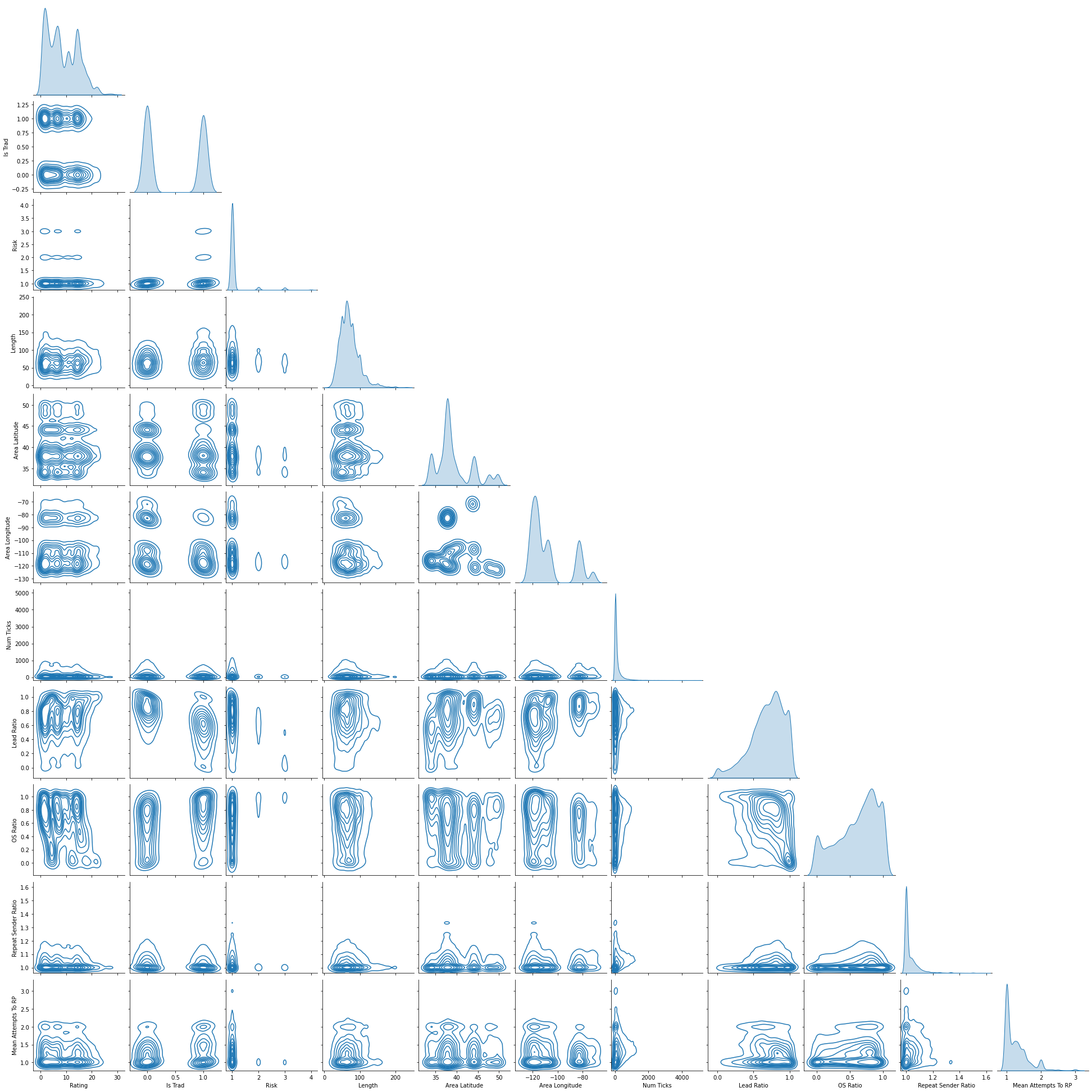KDE Pairplot

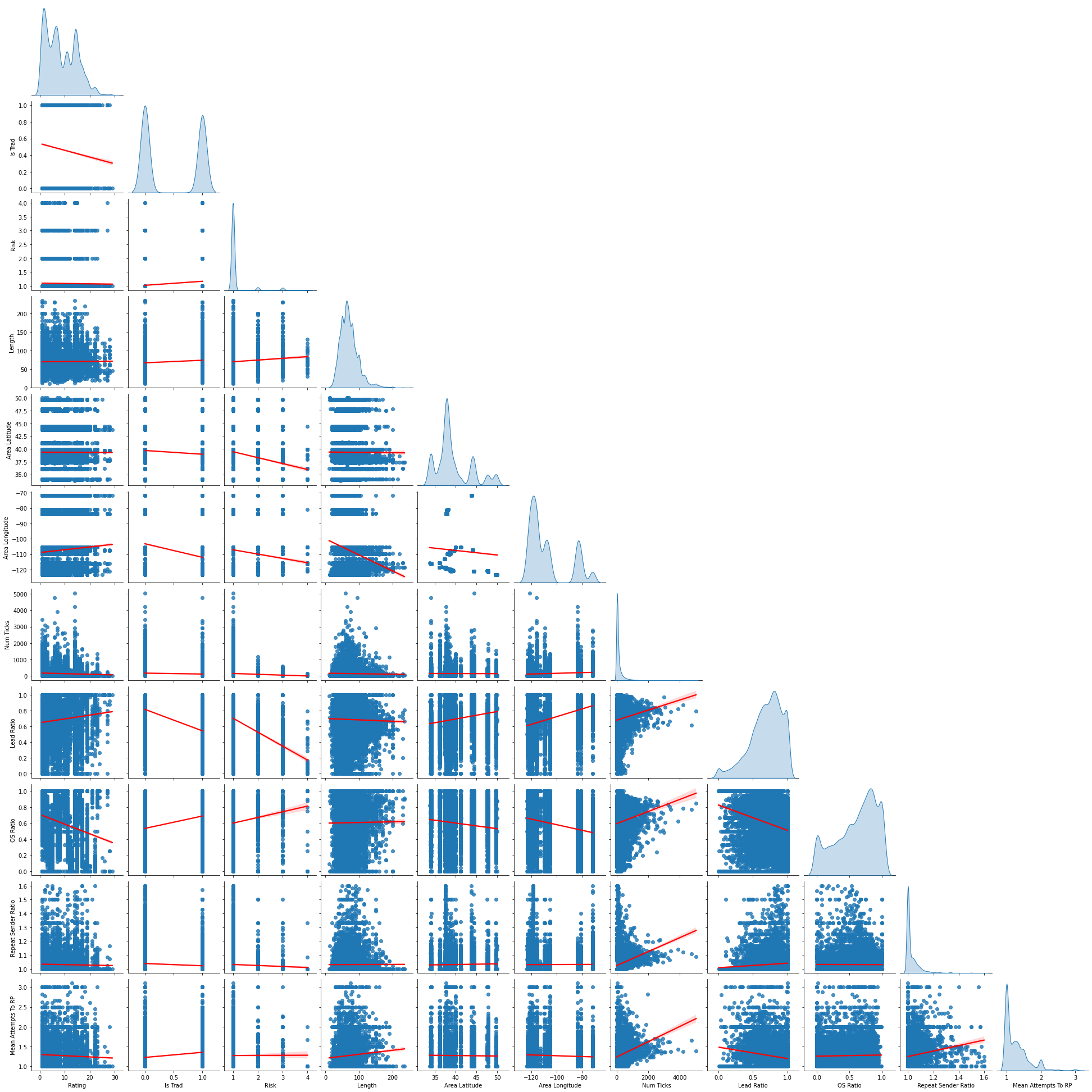Regression Scatter Pairplot

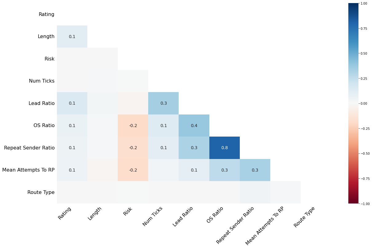
It is also always useful to check a correlation heatmap. 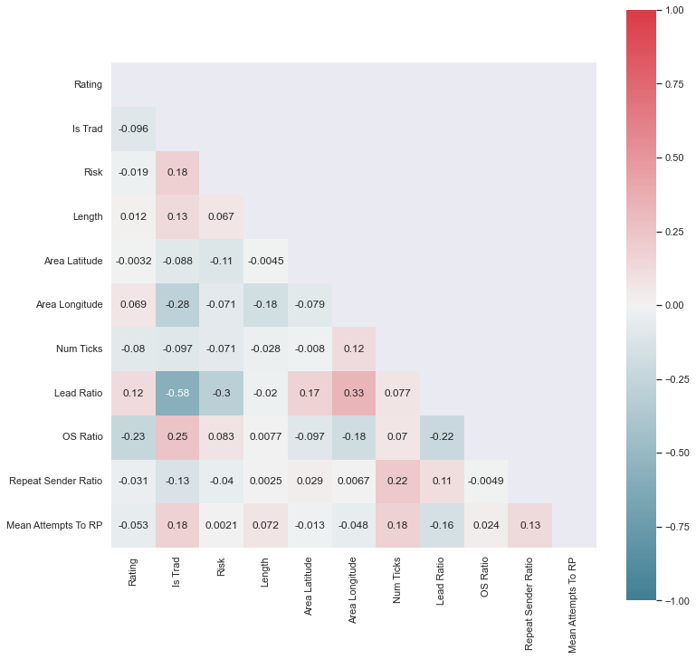Feature Correlation Heatmap

These plots have been commented on in-depth in the previous post, so I will skip that here.

Feature Selection

Our key metric for all of these considerations will be MSE computationally and RMSE for visualization. All use 5-fold cross-validation.

Model Options

We know we are going to perform multiple linear regression. Our choice of type is mostly based on the method of feature selection we want to use.

• Basic Linear Regression with Subset Selection
  • All subset stepwise feature selection - Requires anywhere from 2^11=2,048 to 2^16=65,536 fits. Known to be computationally expensive and here I agree. We will pass on this one.
  • Forward stepwise feature selection - Add features one a time and see if it improves key metric. Does not guarantee the exact best combination of features, but still does a solid job with drastically reduces computational overhead of (p(p+1)/2)+1. In this case 67 to 137.
  • Backward stepwise feature selection - Remove features one at a time and see if it improves key metric. Similar to forward method.
  • Mutual Info Regression - Select the top M features with highest dependency on response variable.
• Dimensional Reduction
  • Principal Component Reduction (PCR) - Construct the first M principal components using standard PCA, and using these components as the predictors for an OLS regression. M to be tuned with cross-validation. Using less features that capture most of the useful information helps to reduce bias.
  • Partial Least Squares (PLS) - PLS sets the principal component directions equal to the coefficient from a simple linear regression. This way, it prioritizes variables that are strongly related to the response. PLS performs this on one predictor, then regresses each variable onto the direction, and takes residuals. We use this orthogonalized residual data to create the next direction. We do this M times, which is a tuning parameter you must select. Where PCR is unsupervised and agnostic to the coefficients we are trying to calculate, PLS takes these into account. For this reason I prefer PLS here and will opt for it instead of PCR.
• Feature Selection with Trees - One can also use a random or boosted forest to identify important features. It is important to eliminate highly correlated features before handing off a feature list to a tree model. Correlated features will be given equal or similar importance, but overall reduced importance compared to the same tree built without correlated counterparts. Random Forests and decision trees, in general, give preference to features with high cardinality. I’ve foregone implementing this method here.

Benchmarking Preprocessing Parameters With Basic Linear Regression

The model may be dependent on our method of three key data preprocessing parameters: categorical encoding, imputation and scaling. We were able to make do with basic encodings which do not have variants to consider. As such, we only need to consider our imputation and scaling methods.

For imputation we effectively have a choice between a simple imputation or a regression imputation and whether or not to include impute indication features AKA “MissingVal Features”. For scaling we have a choice between the five types outlined in the scaling section.

It turns out that the best combination is simple imputation with missingval features in combination with quantile scaling. I would note that a simple imputation without missingval features is only a hair worse and much simpler. This is probably the way to go.

Note that this graph is the difference from the minimized RMSE, calculated as 0.3632. This our baseline value going forward.

	YES Simple Impute | YES MissingVal Features	NO Simple Impute | YES MissingVal Features	YES Simple Impute | NO MissingVal Features	NO Simple Impute | NO MissingVal Features
Standardize	-0.0046	-0.0105	-0.0067	-0.0071
Normalize	-0.0063	-0.0074	-0.0052	-0.0093
Robust	-0.0051	-0.0093	-0.0050	-0.0085
Quant	0.0000	-0.0033	-0.0008	-0.0024

You’ll notice Power Transform is missing here. It didn’t play well with my data even using Yeo-Johnson over Box-Cox. It is sensible to me that Quantile Transformer works as well as it does knowing how outlier prone some of the features may be.

basic_linreg = LinearRegression()
basic_linreg_pipe = Pipeline([('preproc', preproc_pipe), ('model', basic_linreg)])
print(np.mean(np.sqrt(-cross_val_score(basic_linreg_pipe, X_train, y_train, cv=5, scoring='neg_mean_squared_error'))))
print(np.mean(cross_val_score(basic_linreg_pipe, X_train, y_train, cv=5)))

Even though we are not using cross validation to tune a parameter, we can still use it to get a reliable mean value among folds. Because we are not training our data with the cross-validation, there is no need to apply it to our hold-out test set. That conceptual benefit occurs within each fold as it is training and testing among folds.

Interaction and Higher Order Terms

If we include interactions and 2nd order terms in our features, we can reduce the baseline RMSE to 0.3485, a modest improvement.

Forward Stepwise Feature Selection / Mutual Info / Partial Least Squares

Forward stepwise feature selection with a key metric tolerance = 0.001 yields the following features as important:

[Length, Num Ticks, OS Ratio^2, OS Ratio : Repeat Sender Ratio, OS Ratio : Num Ticks, Lead Ratio : Mean Attempts To RP, Length^2, Length : Area Latitude, Length : Num Ticks]

This list is fine but let’s try some more reliable methods.

# SequentialFeatureSelector isn't set up to work with pipelines nicely, so we had to do it semi-manually.
X_train_forward_subselect = preproc_pipe.fit_transform(X_train)
sfs = SequentialFeatureSelector(basic_linreg, n_features_to_select='auto', tol=0.001, cv=5, scoring='neg_mean_squared_error')
sfs.fit(X_train_forward_subselect, y_train)
sfs.get_support()
sfs.transform(X_train_forward_subselect)

Mutual Information gives us the following rough ranking:

This ranking feels relatively fair to me. Certainly Num Ticks and Rating should be up there. I’m surprised that OS Ratio and Repeat Sender Ratio are so high. I expected all of the rest except Length to rank relatively low. These subversions of expectation are in part why this kind of analysis is important.

X_train_mi = preproc_pipe.fit_transform(X_train)

mi_dat = mutual_info_regression(X_train_mi, y_train)
MI_df = pd.DataFrame(data=mi_dat, index=X_train_mi.columns, columns=['MI']).sort_values('MI', ascending=False)
print(MI_df)

mi = SelectKBest(mutual_info_regression, k=50)
mi.fit_transform(X_train_mi, y_train)
mi_support = mi.get_support()
print(mi.transform(X_train_mi).columns)

We will use this method

Partial Least Squares is another solid choice here.

We see that we bottom have a lot to gain going to 10-15, then a bit to gain up to around 30. From then on there is not much more to gain. I’d say ~25 features may well be sufficient here. While our cross validation yields a value of 0.3442, which is a slight improvement of ~0.04 over out benchmark with less than half the features.

X_train_mi = preproc_pipe.fit_transform(X_train)

mi_dat = mutual_info_regression(X_train_mi, y_train)
MI_df = pd.DataFrame(data=mi_dat, index=X_train_mi.columns, columns=['MI']).sort_values('MI', ascending=False)
print(MI_df)

sfs = SelectKBest(mutual_info_regression, k=5)
sfs.fit_transform(X_train_mi, y_train)
sfs.get_support
print(sfs.transform(X_train_mi).columns)

Model Selection

• Regularization (Shrinkage) Methods
  • Ridge - Instead of minimizing least squares, minimize least squares plus a tuning parameter based on the coefficient. Keeps all features in the model, does not perform feature selection. As such not suggested if you believe some of your features may be irrelevant. Can only shrink coefficients asymptotically to zero due to the second power on the shrinkage component (L2 regularization).
  • Lasso - Similar in concept to Ridge Regression, but allows for individual coefficients to be zero as the shrinkage component is first power (L1 regularization). This allows LASSO to effectively perform feature selection. If there are highly collinear variables, LASSO will arbitrarily toss all but one. This may negatively impact interpretability.
  • Elastic Net - Hybrid of both Ridge and Lasso. Has a second parameter that essentially weights each of the regularization methods, with 0 being full Ridge and 1 being full Lasso.
• Outlier Resilient Loss Functions - We can use Huber, RANSAC or Theil-Sen loss functions to reduce the impact of outliers on our model. Since our data has many outliers this can certainly be useful.
• Generalized Linear Models - These are useful if your response variable is not normally distributed. Here ours certainly is, so this is not helpful.
• Stochastic Gradient Descent Regression - This is really just an alternative solver for our regression that may provide performance benefit. Our performance is fine so this is not useful.
• Generalized Additive Models - We can use these to model particularly non-linear relationships. From our EDA our variables look like they can adequately be explained by 1st, 2nd or 3rd order terms.

Regularization Methods

Ridge yields an RMSE of 0.3489. Lasso yields an RMSE of 0.3487, and does not set any feature coefficients to zero. Elastic Net prefers minimal L1 regularization (L1 ratio = 0.001) and just a bit of regularization (alpha=0.0004). It yields an RMSE of 0.3402. The alphas for all of these are near zero suggesting that regularization does not help us too much. This is also clear from the modest gains in RMSE.

ridge = Ridge()
ridge_pipe = Pipeline([('preproc', preproc_pipe), ('feature_sel', mi_feature_sel), ('ridge_model', ridge)])
parameters = {'preproc__scaler': scaler_sel_list, 'feature_sel__percentile':[10,20,40,80], 'ridge_model__alpha':np.logspace(-5, 3, 100)}
ridge_reg= GridSearchCV(ridge_pipe, parameters, scoring='neg_mean_squared_error', cv=5, n_jobs=num_cpu_util)
ridge_reg.fit(X_train, y_train)
print(mean_squared_error(y_test, ridge_reg.best_estimator_.predict(X_test), squared=False))
print(ridge_reg.best_estimator_.score(X_test, y_test))
print(ridge_reg.best_estimator_['ridge_model'].coef_)
print(ridge_reg.get_params)

lasso = Lasso()
lasso_pipe = Pipeline([('preproc', preproc_pipe), ('lasso_model', lasso)])
parameters = {'preproc__scaler': scaler_sel_list, 'lasso_model__alpha':np.logspace(-5, 3, 10)}
lasso_reg= GridSearchCV(lasso_pipe, parameters, scoring='neg_mean_squared_error', cv=5, n_jobs=num_cpu_util)
lasso_reg.fit(X_train, y_train)
print(mean_squared_error(y_test, lasso_reg.best_estimator_.predict(X_test), squared=False))
print(lasso_reg.best_estimator_.score(X_test, y_test))
print(lasso_reg.best_estimator_['lasso_model'].coef_)
print(lasso_reg.best_params_)

elastic = ElasticNet()
elastic_pipe = Pipeline([('preproc', preproc_pipe), ('elastic_model', elastic)])
parameters = {'preproc__scaler': scaler_sel_list, 'elastic_model__alpha':np.logspace(-6, 2, 10), 'elastic_model__l1_ratio':np.linspace(0.001,0.999,10)}
elastic_reg= GridSearchCV(elastic_pipe, parameters, scoring='neg_mean_squared_error', cv=5, n_jobs=num_cpu_util)
elastic_reg.fit(X_train, y_train)
print(mean_squared_error(y_test, elastic_reg.best_estimator_.predict(X_test), squared=False))
print(elastic_reg.best_estimator_.score(X_test, y_test))
print(elastic_reg.best_estimator_['elastic_model'].coef_)
print(elastic_reg.best_params_)

Note that I’ve only implemented feature selection for ridge, as both lasso and elastic net have L2 regularization that enacts feature selection.

Outlier Resilient Loss Functions

I’ve opted to use a Huber loss here. The goal is to see if a reduction in impact of outliers can help our model. Since this model has L2 regularization I’ve omitted feature selection.

huber = HuberRegressor()
huber_pipe = Pipeline([('preproc', preproc_pipe), ('huber_model', huber)])
parameters = {'preproc__scaler': scaler_sel_list, 'huber_model__epsilon':np.linspace(1.35, 10000, 100), 'huber_model__alpha':np.logspace(-6, 2, 10)}
huber_reg= GridSearchCV(huber_pipe, parameters, scoring='neg_mean_squared_error', cv=5, n_jobs=num_cpu_util)
huber_reg.fit(X_train, y_train)
print(mean_squared_error(y_test, huber_reg.best_estimator_.predict(X_test), squared=False))
print(huber_reg.best_estimator_.score(X_test, y_test))
print(huber_reg.best_params_)

With this method we were able to accomplish an RMSE of 0.3623. This method then does not provide a compelling benefit.

Best Method

Elastic Net and PLC Regression are our top contenders. Both of these methods provide an additional benefit in the form of feature selection. An RMSE of 0.3402, which is ~8.5% of our range of 4 for star quality. While this may not enable us to delineate on a high resolution, it does allow us to predict when a route may be particularly bad or good. For many climbers, this may be good enough.

Conclusion

Overall I’m frankly a little disappointed with how little my tinkering improved the model. I suppose this is real data after all, flaws included. I look forward to seeing what a tree-based model can do for us. Ultimately, I think that we simply do not have enough meaningful features to explain all of our variance. If I were really intent on improving this model, I think the hard work is going to come from yielding additional informative features from my data source.