Check Out a Deployed Demonstration of the Model

If you want to check out my code:

Git Repo for model training.

Git Repo for model deployment.

Purpose

Currently on online climbing guidebook websites such as Mountain Project and Open Beta images are typically grouped and assigned to either a location or specific route/problem. Within that initial grouping, there is no further delineation of image type. For a typical user, there are two primary use-cases for the images, information and viewing pleasure.

Information typically comes in the form of what is known as a topographic map, or topo. A topo is either hand-drawn, or a photo with an overlay. A topo helps to locate the route, gauge difficulty, and keep them on the intended path. This is important for both efficiency and safety. It is not uncommon for a climber to reference a topo while on the route, either printed out or on their phone. Whether you’re looking for information on the ground or cliffside, being able to easily access all available information quickly is useful. Currently, the topos are scattered amongst other less helpful images. The ability to classify and group topos together would be a welcome feature.

The other primary purpose of these images is really just to entertain. It is fun to see cool photos. Some photos can inspire one to pursue an objective, or provide nostalgia on a previous experience. Of course not every image is of equal quality. A simple system, currently implemented, is to allow users to rate a photo, and display them in the ranked order. This is effective for popular groupings with exceptionally good (or bad) photos that drive people to go out of their way to vote, but most images exist with little to no user input. Some level of light baseline assertion of quality could go a long way to improving user experience.

Of course determining image quality with a neural network is a nebulous and gargantuan task. So I’ve narrowed in on classifying one particularly pervasive low quality image type. Many shots are taken from below the climber, because fellow climbers are either hanging out at the ground beneath a boulder, or belaying the climber on a route. They are so pervasive because it is the default position, other photos simply require more effort. Because the photo is taken at an angle beneath the climber, oftentimes their legs and rear end block any other part of the subject from view. It is known, tongue-in-cheek, as a “butt-shot”. Other image perspectives often present compelling elements such as facial expression, body positioning and background landscape. These higher quality images I will refer to as a “glory-shot”. Of course it is a matter of opinion, but these butt shots are typically regarded as lower quality. So the goal is to be able to identify these butt-shots. The application of such a classification could for example be to prevent them from showing up as the display image or first provided image for a grouping. This would elevate the overall quality of the website.

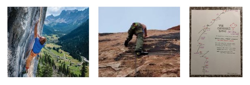A typical glory-shot, butt-shot and topo from left to right

So the overall goal is to train a convolutional neural network to classify an image into one of three categories: glory-shot, butt-shot, topo.

Data Sourcing

Of course there is no standard dataset for this kind of model, so what can you do but make your own. I collected and labeled 3,400 images. It took me about 10 mind numbing hours over two sessions, kept sane by a few This American Life podcasts.

I collected photos from google images and various open-source image banks. I bulk downloaded them with this Chrome Extension. I deleted duplicate images with a quick hash-value script, and got to sorting. I thought about using an image labelling tool, or even making my own quick little GUI, but figured I could just grind through it faster. I primitively used side by side windows file explorer windows and just set the view to extra large preview, and dragged images one by one to dedicated folders each representing a class. Not pretty, but it worked. I then renamed them, and gave them a nice initial shuffle to minimize any underlying trends in the order of my collection.

It’s a common question to ask how much data is enough to start. I had read that ~1000 / class is a good starting point and aimed for that. Past that, it’s more a question of resources and potential benefit. I initially started with ~2,500 images and put together some models. I added another 900 images and did not see much of a performance benefit, so called it there to save my eyes the squinting.

Dealing With Ambiguity in Classes

There is a bit of an issue when it comes to labelling classes in this problem. The idea of what constitutes a topo is pretty cut and dry, it almost always has some sort of symbols, markings or writing to provide some information. However, what constitutes a butt-shot is not certain. There are some images that are able to be classified unquestionably, but there are some that are hard to make heads or tails of.

The solution to this might be to ask multiple people to classify the same data, and assign it a consensus or Bayesian confidence. I’m not subjecting anyone else to labelling so you’re stuck with my interpretation.

Whether to classify an image as a topo is objective. It is either a hand-drawn topo, or an real-world image with overlayed text or symbols. Though what constitutes a butt-shot is pretty clear, there are some examples that seem to be on the borderline.

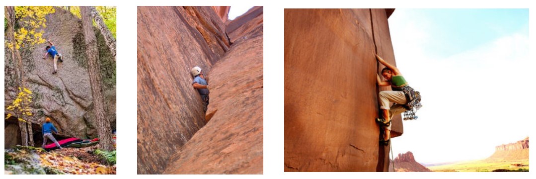Some examples of images where the class is borderline.

This is a tricky and unavoidable issue with how we’ve set up our class definitions. This will make it quite difficult to reach a high (>99%) accuracy. If the model is well trained, then it will output a less-than-confident assertion, say no class probability >90%. We can take these to be effectively an “other” class, which is either irrelevant to the existing three classes, or a borderline case. Then, no grouping can be applied to the image.

Dealing With Imbalanced Data

The volume of data for each class is: 1178 topos, 693 butt-shots, 1179 glory-shots. There are less butt-shots out there than the other types of images (thankfully). If we give our model less images of the under-represented class to train on, it is likely that it will be less capable of correctly classifying them. To ensure that our model is generally capable, we have to do a few important things.

Ensure the training / validation / test data each has the same proportion of classes. That way we are training, validating and testing on datasets that are the same in this critical way.
Amend our batch sampling technique during training to randomly select classes equally so the training model sees a balanced proportion of classes.
Optionally use a loss function that gives more or less weight to the impact of a training image on the model based on class proportion.

Basic Structure of Code

I used PyTorch as the framework for my models and Weights and Biases to manage my training. I used my home computer with an Nvidia 2080 GPU to crunch the numbers.

First we have to load our data, and perform pre-processing image transformations to get it into a usable format.
Then we split the data into training, validation and test data sets. This way we can gauge the performance of the model using data that the model hasn’t already seen, ie. cheating AKA data leakage.
Then we set up a data sampling technique to determine how we will batch data together for each model learning cycle.
Typically a training cycle consists of passing data forward through the model, checking how well it did with a loss function, and back propagating amendments to your model parameters in an attempt to do better next time.
We need to select an appropriate loss function which crunches some numbers to determine how well our model is doing.
We also need to select an appropriate optimizer, which decides how our model is going to try and do better.
We will also consider various learning rate schedules, which is a further tweak to our learning process that can help us find the best possible model.
Of course we need to select a model architecture, and also the details of that architecture.
We must also decide if we will be training a model from the ground up, using a pre-trained model as a fixed feature extractor, or re-train a pre-trained model.
I used early stopping logic is really useful to prevent wasted time on models that are unlikely to turn up anything of value.
I created some utility functions to save the best model, save mislabeled images for inspection, and provide precision/recall/f1 values for all classes.
Weights and Biases was critical to effective hyper-parameter sweeping and model analysis. It saved me a lot of time and headache, I’m a huge fan.

Image Preprocessing

I began by down-sampling the images of various resolutions down to a consistent 224x224 resolution. This matches the resolution of the images that pre-trained models are trained on, which is helpful but not necessary. More importantly it allows me to efficiently fit a handful of images at once onto my GPU VRAM, otherwise training would slow to a crawl.
I also normalized the image to the imagenet normalization Mean = [0.485, 0.456, 0.406] STD = [0.229, 0.224, 0.225] This is useful if we are to use a model pre-trained on imagenet data.
I also added some optional transformations as a hyperparameter, including a random horizontal flip and color jitter.

Data Splitting

We divide our dataset into:

A training set used to actually develop the model.
A validation set used to ascertain the quality of the model at each step of training, using data that the model has not seen.
A test set that is used a final metric of quality for a given model. This is also data that the model has not seen before.

I used an 80/10/10 split for train/validation/test. The more training data the better, but if you don’t leave enough data for validation and testing, your guiding metrics may misguide you.

Again, we split it using stratification so class proportion is preserved amongst the split.

Data Sampling

One critical decision to be made is how much data to feed the model each learning cycle. You can do it one at a time, but it may take a long time. You could try and pass as much as possible, but you are limited by your GPU capacity. Batch size is commonly taken to be some value of 2ⁿ, typically 16, 32, 64 etc.

My GPU was saturated around a batch size of 64, so I took that to be the upper limit.

It helps training stability to have some of each class in a batch, so I wouldn’t want to go much below 8 to be safe.

Again, we use a weighted random sampler to ensure equal training exposure of each class for each batch.

Loss Function

For multiple class image classification, Cross Entropy Loss is the go to, and I did not find a compelling reason to try anything else.

I did provide an optional weighted cross entropy loss if I believed class imbalance to still be an issue.

Optimizer

Adam Optimizer seems to be a fan favorite, and I’m no different. It performed very nicely for me out of the box. I would consider using a more tightly tuned SGD optimizer, but ended up being happy enough with Adam to not try it. There’s enough tweaking required to get a good learning rate schedule, it was nice not to have to mess around with the optimizer in addition.

Learning Rate Schedule

I used the excellent Learning Rate Range Test to obtain appropriate magnitudes by which to sweep. This was most useful in avoiding learning rates that result in unstable high loss.

I tried a few different schedules:

A basic constant learning rate.
Exponential decay.
OneCycle.
Cosine Annealing with Warm Restart.

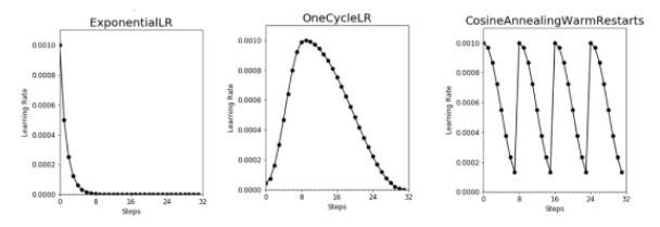Visualizations of the various learning schedules

Model

I began with a very basic LeNet architecture to get off the ground. I explored various architecture parameters with varying levels of success, obtaining up to a 79% test accuracy, not bad!

I soon moved onto a slightly more complex AlexNet architecture with similar levels of success.

I moved onto using imagenet pre-trained models. I found that retraining the whole model provided a 1-5% accuracy boost compared to using them as a fixed feature extractor. I found that I could quickly achieve ~90% accuracy. Conceptually and functionally I’m a big fan of these pre-trained models. Stand on the shoulders of giants whenever possible.

I tried all sorts of models such as:

AlexNet
VGG11, VGG16
ResNet18, ResNet50
DenseNet121
SqueezeNet1_1
MobileNet_v3_Large

In general I found AlexNet modestly underpowered compared to the others. I found that VGG11 and ResNet18 provided me the best balance of complexity and performance. The other models were quite a bit more expensive to train, and provided little if any benefit to my application.

Model Checkpointing

I used a basic function to compare validation accuracy between epochs. If the accuracy is better at a given epoch, the model parameters are saved as the “best model”. Once all epochs are complete, I save the best model for potential use later. This model is also used on the hold-out test data for our final test accuracy metric.

Additional Run Output Metrics

I wrote a small function that saves all incorrectly labelled images in a folder structure that is first the correct label, then the incorrect label assigned to it. In this way I can quickly scan for commonalities between incorrectly labelled images. I found that most of the time the assigned label itself was borderline as mentioned in the previous section “Ambiguity in Classes”.

I also wrote a small utility script to output a precision, recall, and f1 score for each class. In this way I can further delineate model performance on a class by class basis. It also told me that generally topo and glory are quite easy to get a high accuracy for, and butt-shot is the most difficult. This is logical to me because topos have very obvious features to pick up on, such as high contrast colored symbol overlays and text. Glory shots typically have faces and landscape features to go off of. Butt-shots have the aforementioned ambiguity issue.

Early Stopping

If my training destabilized, I would sometimes see the model settle into guessing a single class no matter what, and be unable to learn it’s way out of it. To prevent me from wasting time on these hopeless models, I established some early stopping logic to detect this and log a flag if it were to occur.

I found that often it was a hyper-parameter that would incur destabilization of the training such as a high learning rate. I also found that using both weighted random sampling and weighted cross entropy was often not a good idea. Since weighted random sampling already “fixed” the class imbalance issue, adding weighted cross entropy in addition doubled down on the effect, which resulted in over-weighting of the imbalanced class. This is supported by the fact that the vast majority of single guess models were guessing the low-volume class.

With iterative sweeps, I was able to bound the sweep domain tighter and tighter to avoid this from happening.

Settling on a Model

Squeezing Out Extra Performance With Hyper-Parameter Sweeps

I was lucky enough that the pre-trained models performed quite well out of the box, yielding a validation accuracy of >80% typically in the first few epochs. This usually ended up settling in the 92%-96% in <30 epochs for most “good” models.

Below we can see that our models exhibit typical loss behavior, with validation loss bottoming out and then increasing, while training loss continues to asymptote. This typically signifies overfitting, and is the reason we checkpoint the best model.

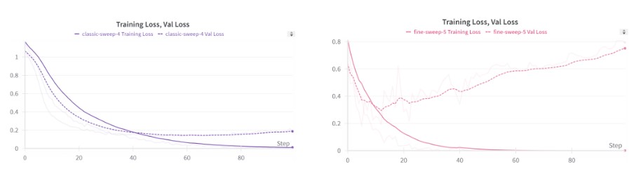Two examples of training/validation loss curves.

For the most part I used random searching. Once I had my hyper-parameter space iteratively pruned, I used a full grid search to lock in the best performing model.

When looking at the sweep output, we can begin to discern what hyper-parameters matter, and in what way. In general, we are looking for imbalanced groupings of pinkish lines which signify a poorly performing parameter.

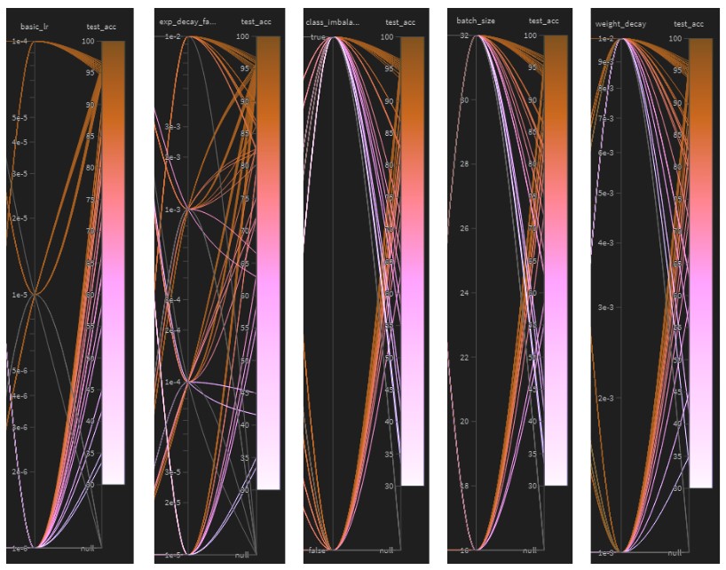Various parallel plots

Too small of a learning rate is bad. This is likely because the model does not then have time to find it’s absolute minimum since the number of epochs is the same among runs.
It seems that a larger exponential decay factor is helpful. Exponential decay factor is the proportion of the initial learning rate that the schedule will drop to. This shows that perhaps we do not want to drop our learning rate too fast.
Class Imbalance Loss tends to hurt us. This is because we already have weighted random sampling enabled, and this then over-weights imbalanced classes.
Batch size has a modest negative impact, but the training efficiency benefit may be worth it depending on the application.
The degree of weight decay looks to have little impact, but I know from early sweeps that some weight decay is helpful.

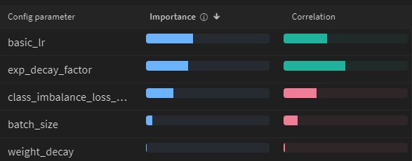Sweep correlations for various hyper-parameters in relation to test accuracy.

My Best Model

Ultimately, my best hyper-parameters were:

Parameter	Value	Description
Pre-Train Model Type	VGG11	Base model architecture, AlexNet, VGG11, Resnet Etc.
Pre-Train Type	Full Re-Train	Full re-train or fixed feature extractor.
Epochs	50	Number of epochs
Batch Size	32	Batch size of mini-batched sampling method.
Starting Learning Rate	0.0001	Learning rate at first epoch.
Learning Rate Schedule Type	Exponential Decay	Constant, Exponential Decay, OneCycle, Cosine Anneal w/ Warm Restarts
Exponential Decay Factor	0.01	Proportion of starting LR to decay to.
Weight Decay	0.001	Weight decay added
Dropout	0.5	Dropout proportion in added fully connected layer.
Complex Image Transform	FALSE	Random flipping and color jitter.
Class Imbalance Split Handling	TRUE	Stratified data splitting.
Class Imbalance Sample Handling	TRUE	Weighted random sampling
Class Imbalance Loss Handling	FALSE	Weighted cross entropy loss

The class accuracy, precision and F1 are as follows:

Class	Precision	Recall	F1
Glory-Shot	0.984	0.954	0.969
Butt-Shot	0.925	0.961	0.943
Topo	0.977	0.984	0.981

My final test accuracy was 96.7% and loss was 0.25

Model Deployment Pains

I deployed a demonstration of my model using streamlit. The main issue I had was dealing with how large the .pth file was. I wanted to avoid having to use git large file storage and potentially needing to pay for storage. That means the file had to be <100Mb but it was 500+.

I tried to zip it, but that only reduced it by ~5%.

I tried quantizing the file from float32 to int8, which cut the file size to a quarter, but it was not enough.

I thought about pruning, but figured I would have to prune quite a bit of my model. I would also need to tune my pruning based on performance, which would be quite a bit of effort.

I was already at the limit of free storage from past large file commits. I ended up taking the easy way out and just paid the $5 so I could upload the large file. The model still performed quite fast, so that was not a concern once deployed.

I figured I could pay for one month of data, and cancel it. But once you are above the data alloted, you need to be below the quota to reduce your payment plan. The large files I needed would be below the quota, but large files in your commit history count against your quota even if they aren’t in your most current commit! So I had to break out the git scalpel and purge my commit history of these parasitic large files, and even reach out to customer support to have them delete it on their end. The only alternative was deleting and re-initializing the repo which would lose me all of my commit history. It was a wildly inconvenient process that I was not expecting. I suppose there is something to learn from every git battle.

Other Lessons Learned

I learned what level of model improvement to expect from hyperparameter optimization. It was frankly less than I was expecting, and often dependent on a few critical parameters. I suppose this is where the artisanry of model development comes from.
I really enjoyed using Weights and Biases. Being able to watch runs progress and set up sweeps was critical to obtaining a performant model in a reasonable amount of time.
Data acquisition is the hard part. Tuning a model is pretty fun, but labelling data or having to pay someone else to do it for you is much less fun.
I was able to get a very good feel as to what effect various parameter values will have on the model.
Learning rate scheduling felt very impactful to the overall training experience in terms of performance and required runtime. I’m looking forward to obtaining a better intuition and control over this important parameter.
Early stopping is really nice to reduce overall training time efficiency. It is well worth the effort.
It doesn’t feel right at first, but random searching really is much better than grid searching for any wide parameter domain. I was impressed with the amount of speedy intuition I was able to build.
Class imbalance issues can really hurt you. How you handle them has a large impact on your model.
If you’re going to be storing large files, you should have your credit card ready. Being able to educe file size with quantization and pruning without sacrificing performance is a worthwhile skill.

Training a Convolutional Neural Net For Climbing Image Classification